9702/May Jun/12/2015/Q6

A single sheet of aluminium foil is folded twice to produce a stack of four sheets. The total thickness of the stack of sheets is measured to be (0.80 ± 0.02) mm. This measurement is made using a digital caliper with a zero error of (−0.20 ± 0.02) mm.

What is the percentage uncertainty in the calculated thickness of a single sheet?

A 1.0%                        B 2.0%                        C 4.0%                        D 6.7%

Solution:

Answer: C

This challenging question involves both random and systematic error.

The zero error (−0.20) can be removed but its uncertainty (± 0.02) must be added to the measurement uncertainty.

True value of total thickness = 0.80 + 0.20 = 1.0 mm  

Total uncertainty in measurement = ± (0.02 + 0.02) = ± 0.04

So the four sheets have a true thickness of (1.00 ± 0.04) mm.

A single sheet would have a thickness of (0.25 ± 0.01) mm.

Percentage error = (0.01 / 0.25) × 100% = 4%

Reference: PYQ - Oct/Nov 2015 Paper 12 Q6

9702/May Jun/11/2011/Q5

The diagram shows an experiment to measure the speed of a small ball falling at constant speed
through a clear liquid in a glass tube.

There are two marks on the tube. The top mark is positioned at 115 ± 1 mm on the adjacent rule
and the lower mark at 385 ± 1 mm. The ball passes the top mark at 1.50 ± 0.02 s and passes the
lower mark at 3.50 ± 0.02 s.

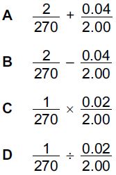
The constant speed of the ball is calculated by (385 – 115) / (3.50 – 1.50) = 270 / 2.00 = 135 mms^-1.

Which expression calculates fractional uncertainty in the value of this speed?

Solution:
Answer: A

Speed v = Distance s / Time t

Δv / v = (Δs / s) + (Δt / t)

Fractional uncertainty of speed = Δv / v

Distance s = 385 – 115 = 270 mm

Δs = ± (1 + 1) = ± 2 mm

Time t = 3.50 – 1.50 = 2.00s

Δt = ± (0.02 + 0.02) = ± 0.04 s

Reference: PYQ - May/Jun 2011 Paper 11 Q5

9702/Oct Nov/11/2015/Q4

A calibration graph is shown for an ammeter whose scale is inaccurate.

Two readings taken on the meter at different times during an experiment are 0.13 mA and
0.47 mA.

By how much did the current really increase between taking the two readings?

A 0.30 mA
B 0.35 mA
C 0.40 mA
D 0.44 mA

Solution:
Answer: A

When ammeter reading = 0.13mA, the current = 0.14mA
When ammeter reading = 0.47mA, the current = 0.44mA
The current increase between taking the two reading is 0.44mA - 0.14mA = 0.3mA

Reference: PYQ - Oct/Nov 2015 Paper 11 Q4

9702/Oct Nov/11/2015/Q6

A light-meter measures the intensity I of the light incident on it. Theory suggests that I varies
inversely as the square of the distance d.

Which graph of the results supports this theory?

Solution:
Answer: C

Theory suggests that the intensity I varies as the inverse square of the distance d.

I α 1 / d²

I = k (1 / d²) = k / d²    where k is a constant

Consider the graph of I (on y-axis) against 1/d² (on x-axis).

Equation of a line: y = mx + x

Compare I = k (1 / d²) = k / d² with the equation y = mx + c:

y = I

x = 1 / d²

m = k

c = 0

So, if a graph of I against 1/d² is plotted, it should be a straight line with a positive gradient (the constant k is positive) and starting at the origin (y-intercept, c = 0 – that is, it intercepts the y-axis at y=0). [C is correct]

Options A and B both have the graph cutting an axis, which would not be the case for an inverse square law graph.

A graph of I against d² would be similar to a graph of y = 1 / x where y = I and x = d². Such a graph is a curve with a negative gradient and not touching the axes.

Type: graph y=1/x

at Google search to see to shape of the graph.

Reference: PYQ - Oct/Nov 2015 Paper 11 Q6